静态词向量预训练模型

^ _ ^

Pre-trained Word Vector Task

Given a text $w_1w_2\cdots w_n$, the basic task of language model is to predict the possibility of one word occures in one position. In other word, calculating conditional probablity $P(w_t|w_1w_2\cdots w_{t-1})$.

To consturct Language Model, we can transfer the problem to a classification problem: the input is history word sequence($w_{1:t-1}$), the output is $w_t$. Then, we can use text which is non-labeled to consturct training dataset and train the model by optimizer loss function in this dataset. Since the supervised signal came from the data itself, this type of learning is also called Self-supervised Learning.

Feed-forward Neural Netword Language Model

Bias Hypothesis: Markov Assumption
The prediction of the next word is only associated with the most recent n-1 word in history.
Formually: $P(w_t|w_{1:t-1}) = P(w_t|w_{t-n+1:t-1})$

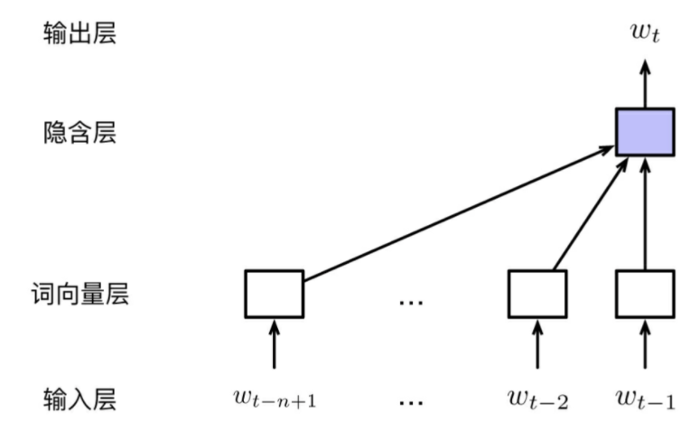
(1) Input Layer: In the current time $t$, every input is composed of history word sequence $w_{t-n+1:t-1}$. Specifically, we can use One-Hot Encoding or Vocabulary Index to present a word.

(2) Embedding Layer: Embedding Layer maps every word in input layer to a dense vector which called feature vector. In other view, Embedding Layer can be viewed as a Look-up Table. The process of get word vector can be viewed as a process of search the vector in Look-up Table according to the index of the word.
Formually, $x = [v_{w_{t-n+1}}; \cdot; v_{w_{t-2}};v_{w_{t-1}}]$, where

• $v_w \in R^d$: shows the word vecotr of d dimenion
• $x \in R^{(n-1)d}$: shows the result of concating all the word vector in history sequence.

We can define word vector matrix $E \in R^{d \times |V|}$, where $V$ is the vocabulary.

(3) Hidden Layer: Linear Transform and Activation to $x$ in Embedding Layer. $h=f(W^{hid}x + b^{hid})$.

• For Linear transform, $W^{hid} \in R^{m \times (n-1)d}$ is the linear transformation matrix from embedding layer to hidden layer.
• For Activation, normally activation function contains Sigmoid, tanh, ReLU.

(4) Output Layer: Linear Transform and Softmax to get probability distribution of Vocabulary. $y = Softmax(W^{out}h + b^{out}$, where $W^{out} \in R^{|V| \times m}$ is the linear transforamtion matrix from hidden layer to output layer.

From what has been discussed above, the parameters of FNN can be represented as $\theta = {E, W^{hid}, b^{hid}, W^{out}, b^{out}}$. The number of parameters is $|V| \times d + m \times (n-1)d + m + |V| \times m + |V|$. And in case of $m$ and $d$ are constant, so the number of parameter will increase linearly according to the size of vocabulary.

Besides, the optimization of hyperparameter such as dimension of word vector d, hidden units dimension m, input sequence length n-1, should be modified by the development dataset.

After the training, matrix $E$ will be the Static Word Vecotr which is pre-trained.

Recurrent Nerual Network Language Model

In the FNN LM, the prediction of next word is depended by the length of history be looked back(parameter n). But in the reality situation, the expectation of n is different because of the different length of sequences. For example, “我吃_“, the word in “_“ should be food can be infered by “吃”, only considering short history. But “他感冒了，于是下班之后去了_“, the word in “_“ should be hospital can be infered by “感冒”, that needs to consider long history.

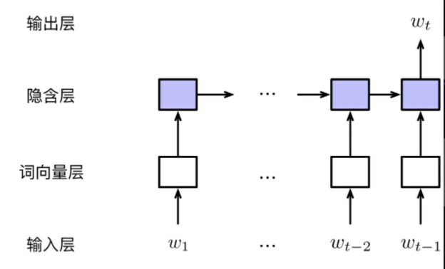
RNN LM has a good nature to deal with the dependency relationship which has unfixed length. RNN maintains a hidden state, which is called Memory, contains all the history information of current word in every moment. Memory and current word will joint together as the input of the next time.

(1) Input Layer: the input in RNN LM is not limited by the window length n any more. It can be represented by the whole history sequence, $w_{1:t-1}$.

(2) Embedding Layer: Like FNN LM, in the Embedding Layer, the input sequence should map to word vector. In RNN, every input of time t should be composed of 2 part: Memory, hidden state $h_{t-1}$; the previous word $w_{t-1}$. Specifically, we add start tag <bos> as $w_0$; zero vector as init hidden state $h_0$. The input of t can be represented as $x_t= [v_{w_{t-1}}; h_{t-1}]$.

(3) Hidden Layer: Like FNN LM, the calculation of Hidden Layer is composed of Linear Transform and Activation Function. $h_t = tanh(W^{hid}x_t + b^{bid})$, where $W_{hid} \in R^{m \times (d+m)}, b^{hid} \in R^m$. For detailed, $W^{hid}=[U; V]$, where $U \in R^{m \times d}, V \in R^{m \times m}$. So another formula has the same meaning, $h_t = tanh(Uv_{w_{t-1}} + Vh_{t-1} + b^{hid})$.

(4) Output Layer: $y_t = Softmax(W^{out}h_t + b^{out})$, where $W^{out} \in R^{|V| \times m}$.

When the input sequence is too long, Vanishing Gradient and Exploding Gradient might occurred. To deal with this problem:

• Before 2015, Truncated Back-propagation Through Time is the mainstream method.
• After 2015, Gating Mechanism is the mainstream method.(e.g. LSTM)

Code

Load Data

load corpus and create vocab

BOS_TOKEN = "<bos>" # sentence head tag
EOS_TOKEN = "<eos>" # sentence tail tag
PAD_TOKEN = "<pad>" # space padding

def load_reuters():
    '''
        reuters is a corpus database which applies to text classification
        including 10788 newspaper documents, which have 1 or more classify label.
    '''
    from nltk.corpus import reuters
    text = reuters.sents()
    text = [[word.lower() for word in sentence] for sentence in text]
    vocab = Vocab.build(text, reserved_tokens=[PAD_TOKEN, BOS_TOKEN, EOS_TOKEN])
    corpus = [vocab.convert_tokens_to_ids(sentece) for sentence in text]
    return corpus, vocab

def get_loader(dataset, batch_size):
    return DataLoader(dataset, batch_size, collate_fn=dataset.collate_fn, shuffle=True)

FNN

create dataset for FNN

class NGramDataset(Dataset):
    def __init__(self, corpus, vocab, context_size=2):
        self.data = []
        self.bos = vocab[BOS_TOKEN]
        self.eos = vocab[EOS_TOKEN]
        for sentence in tqdm(corpus, desc="Dataset Construction"):
            sentence = [self.bos] + sentence + [self.eos]
            if len(sentence) < context_size:
                continue
            for i in range(context_size, len(sentence)):
                context = sentence[i-context_size:i]
                target = sentence[i]
                self.data.append((context, target))
    def __len__(self):
        return len(self.data)
    def __getitem__(self, i):
        return self.data[i]
    def collate_fn(self, examples):
        inputs = torch.tensor([ex[0] for ex in examples], dtype=torch.long)
        targets = torch.tensor([ex[1] for ex in examples], dtype=torch.long)
        return (inputs, targets)

FNN LM

class FeedForwardNNLM(nn.Module):
    def __init__(self, vocab_size, embedding_dim, context_size, hidden_dim):
        super(FeedForwardNNLM, self).__init__()
        self.embeddings = nn.Embedding(vocab_size, embedding_dim)
        self.linear1 = nn.Linear(context_size * embedding_dim, hidden_dim)
        self.linear2 = nn.Linear(hidden_dim, vocab_size)
        self.activate  = F.relu
    def forward(self, inputs):
        embeds = self.embeddings(inputs).view((inputs.shape[0], -1))
        hidden = self.activate(self.linear1(embeds))
        output = self.linear2(hidden)
        log_probs = F.log_softmax(output, dim=1)
        return log_probs

Training

embedding_dim = 128
hidden_dim = 256
batch_size = 1024
context_size = 3
num_epoch = 10

corpus, vocab = load_reuters()
dataset = NGramDataset(corpus, vocab, context_size)
data_loader = get_loader(dataset, batch_size)

nll_loss = nn.NLLLoss()
model = FeedForwardNNLM(len(vocab), embedding_dim, context_size, hidden_dim)
model.to(device)

optimizer = optim.Adam(model.parameters(), lr=0.001)

model.train()
total_losses = []
for epoch in range(num_epoch):
    total_loss = 0
    for batch in tqdm(data_loader, desc=f"Training Epoch {epoch}"):
        inputs, targets = [x.to(device) for x in batch]
        optimizer.zero_grad()
        log_probs = model(inputs)
        loss = nll_loss(log_probs, targets)
        loss.backward()
        optimizer.step()
        total_loss += loss.item()
    print(f"Loss: {total_loss:.2f}")
    total_losses.append(total_loss)

Save model

def save_pretrained(vocab, embeds, save_path):
    with open(save_path, "w") as writer:
        writer.write(f"{embeds.shape[0]} {embeds.shape[1]}\n")
        for idx, token in enumerate(vocab.idx_to_token):
            vec = " ".join([f"{x}" for x in embeds[idx]])
            writer.write(f"{token} {vec}\n")

save_pretrained(vocab, model.embeddings.weight.data, "ffnnlm.vec")

RNN

create dataset for RNN

class RnnlmDataset(Dataset):
    def __init__(self, corpus, vocab):
        self.data = []
        self.bos = vocab[BOS_TOKEN]
        self.eos = vocab[EOS_TOKEN]
        self.pad = vocab[PAD_TOKEN]
        for sentence in tqdm(corpus, desc="Dataset Construction")
            input = [self.bos] + sentence
            target = sentence  + [self.eos]
            self.data.append((input, target))
    def __len__(self):
        return len(self.data)
    def __getitem__(self, i):
        return self.data[i]
    def collate_fn(self, examples):
        inputs = [torch.tensor(ex[0]) for ex in examples]
        targets = [torch.tensor(ex[1]) for ex in examples]
        # padding for different length sequence
        inputs = pad_sequence(inputs, batch_first=True, padding_value=self.pad)
        targets = pad_Sequence(targets, batch_first=True, padding_Value=self.pad)
        return (inputs, targets)

create RNN model

class RNNLM(nn.Module):
    def __init__(self, vocab_size, embedding_dim, hidden_dim):
        super(RNNLM, self).__init__()
        self.embeddings = nn.Embedding(vocab_size, embedding_dim)
        self.rnn = nn.LSTM(embedding_dim, hidden_dim, batch_first=True)
        self.output = nn.Linear(hidden_dim, vocab_size)
    def forward(self, inputs):
        embeds = self.embeddings(inputs)
        hidden, _ = self.rnn(embeds)
        output = self.output(hidden)
        log_probs = F.log_softmax(output, dim=2)
        return log_probs

Training

embedding_dim = 128
hidden_dim = 256
batch_size = 1024
num_epoch = 10

corpus, vocab = load_reuters()
dataset = RnnlmDataset(corpus, vocab, context_size)
data_loader = get_loader(dataset, batch_size)

nll_loss = nn.NLLLoss(ignore_index=dataset.pad)
model = FeedForwardNNLM(len(vocab), embedding_dim, hidden_dim)
model.to(device)

optimizer = optim.Adam(model.parameters(), lr=0.001)

model.train()
total_losses = []
for epoch in range(num_epoch):
    total_loss = 0
    for batch in tqdm(data_loader, desc=f"Training Epoch {epoch}"):
        inputs, targets = [x.to(device) for x in batch]
        optimizer.zero_grad()
        log_probs = model(inputs)
        loss = nll_loss(log_probs.view(-1, log_probs.shape[-1]), targets.view(-1))
        loss.backward()
        optimizer.step()
        total_loss += loss.item()
    print(f"Loss: {total_loss:.2f}")
    total_losses.append(total_loss)

Since the goal of training is to acquire the word vector rather than language model itself. In the training process, it is not necessary to take the convergency state of the model as the termination condition of training.