多层感知机

^ _ ^

The Composition of MLP

Multi Layer Perceptron, named MLP. It is a solution to the linear indivisible problem. Specifically, it can be prepresented by stacking multiple layer Linear Regressioner, and adding Activation Function between layers.

Linear Regression

Standard Linear Regression Model:
$y = w_1x_1 + w_2x_2 + \cdots + w_nx_n + b = wx + b$

Standard Linear Regression Model can solve regression problems, which is to predict continues values. We can also solve classification problem by simply adding threshold choose layer behind the output of y.
e.g.

$$y= \left\{\begin{matrix} 1, & w \cdot x + b \geq t \\ 0, & otherwise \end{matrix}\right. $$

There are two import problem need to be solved when using linear regression:

1. Feature Extraction: Raw Input –> Vector x
2. Parameter Learning: How to choose the fittest param w, b

Activation Function

The codomain of the output of linearn function is infinite, sometimes we need to limit the codomain to a fixed range. Many functions can satisfy the demands.

Logistic

$y = \frac{L}{1+e^{-k(z-z_0)}}$

Properties:

1. The function can limit the codimain of y in the range (0, L)
2. k control the steep degree of the function.
3. When $z = w \cdot x + b$, we named it Logistic Regression Model.
4. When $L = 1, k = 1, z_0 = 0$, we named it Sigmoid Function.
   • The derivative of Sigmoid Function is $y^{‘} = y(1-y)$, which is convenient for params optimization.

Softmax

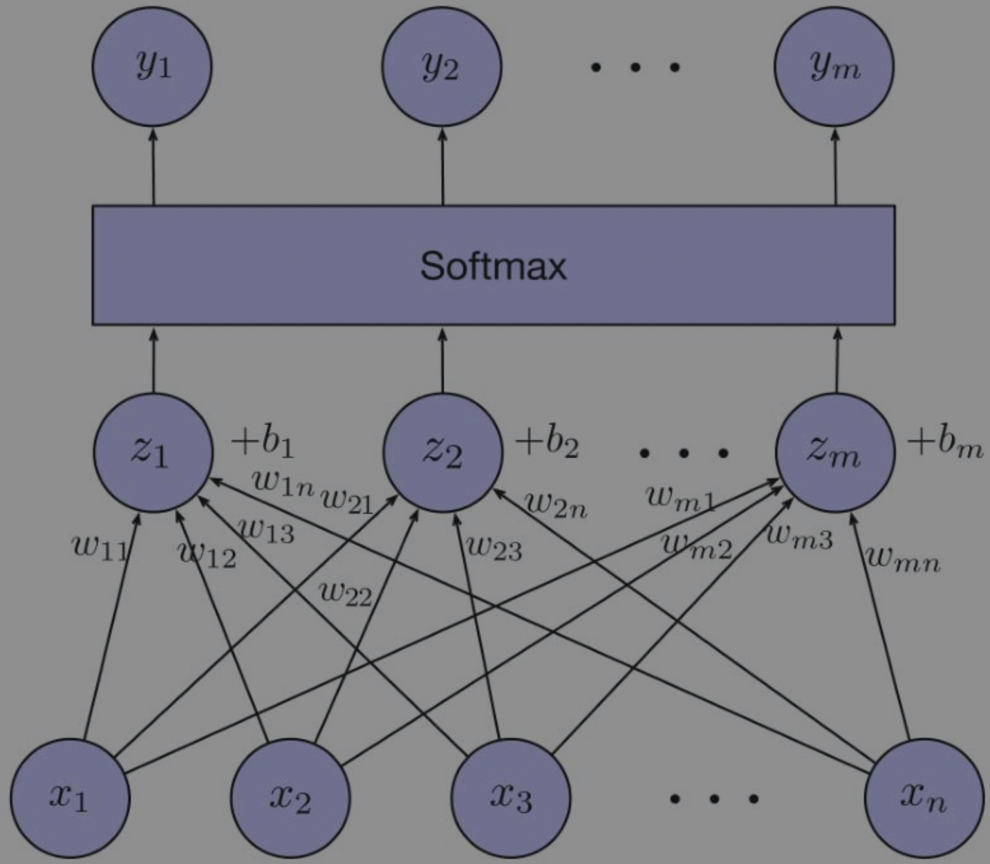
Sigmoid Function can only deal with binary classfication, while Softmax Regression can solve multiple classfication.

$y_i = Softmax(z)_i = \frac{e^{z_i}}{e^{z_1} + e^{z_2} + \cdots + e^{z_m}}$

$z = [z_1, z_2, \cdots, z_m]$, where $m$ is the number of categories; $y_i$ is the probability of category i; $z_i = w_{i_1}x_1 + w_{i_2}x_2 + \cdots w_{i_n}x_n + b_i$

$y = Softmax(Wx + b)$ can matrixly represent as:

ReLU

$ReLU(z) = max(0, z)$

Multi-Layer Perceptron

Combine Linear Regressor and Activation Function, we can design MLP to solve non-linearity problem.

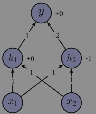
For example, a XOR problem can be solved by MLP with 1 hidden layer.

$$ \begin{matrix} z = W^1 x + b^1 \\ h = ReLU(z) \\ y = W^2h + b^2 \end{matrix} $$

where

$$ W^1 = \begin{bmatrix} 1 & 1\\ 1 & 1 \end{bmatrix}, b^1 = [0, -1]^T, W^2 = [1, -2], b^2 = [0] $$

The more hidden layers, the stronger presentation skills and the more difficult to learn. So we need to find the balanced point between model scale and learning difficulty.

MLP Code

Linear Model

Create a Linear Model

from torch import nn
linear = nn.Linear(in_features, out_features)

Generally, we might input multiple examples at once, which called batch. So the dimension of inputs can be (batch, in_features). In the same way, the dimention of outputs can be (batch, out_features)

# in_features=32, out_features=
linear = nn.Linear(32, 2)
inputs = torch.rand(3, 32)
outputs = linear(inputs)

Activation Function

from torch.nn import functional as F
activation = F.sigmoid(outputs)
activation = F.relu(outputs)
activation = F.softmax(outputs, dim=1) # dim represents the axis 
activation = F.tanh(outputs)

There are 3 ways to use activation function:

1. torch.sigmoid()
2. torch.nn.functional.sigmoid()
3. torch.Sigmoid

1,2 is a function, while 3 is a class. So 1, 2 can use directly, but 1 is preferred. When use 3, you should init it first, then use it.

Custom MLP

import torch
from torch import nn

class MLP(nn.Module):
    def __init__(self, input_dim, hidden_dim, output_dim):
        super(MLP, self).__init__()
        self.linear1 = nn.Linear(input_dim, hidden_dim)
        self.activation = torch.nn.ReLU()
        self.linear2 = nn.Linear(hidden_dim, output_dim)
        self.softmax = torch.nn.Softmax(dim=1)
        
    def forward(self, inputs):
        hidden = self.linear1(inputs)
        activation = self.activation(hidden)
        output = self.linear2(activation)
        probs = self.softmax(output)
        return probs
    
if __name__ == "__main__":
    mlp = MLP(input_dim=4, hidden_dim=5, output_dim=2)
    inputs = torch.rand(3, 4)
    probs = mlp(inputs)
    print(probs)